Follow a velocity field.
Learn local dynamics along a noise-to-data path. Numerical integration offers a natural way to spend more computation at inference.
NeurIPS 2026
One-step generation.
Flexible multi-step refinement.
1 UC Irvine2 University of Virginia3 University of Alabama at Birmingham4 Northeastern University
Can a drifting generative model keep its direct, one-step generation and also benefit from more inference steps? DFM learns transport between intermediate distributions, making both choices available to the same model.
01 / The problem
Flow-based and drifting models offer different ways to turn noise into data. The paper asks how to connect their inference behavior.
Learn local dynamics along a noise-to-data path. Numerical integration offers a natural way to spend more computation at inference.
Use distribution-level drift during training to shape generated samples. A direct endpoint map supports one-step generation, but does not naturally specify intermediate inference steps.
Apply drift supervision between intermediate marginals. The learned transport can span the whole path in one call or compose shorter intervals.
02 / The mechanism
The probability path comes from Flow Matching. The learning signal is a distribution-level drift correction.
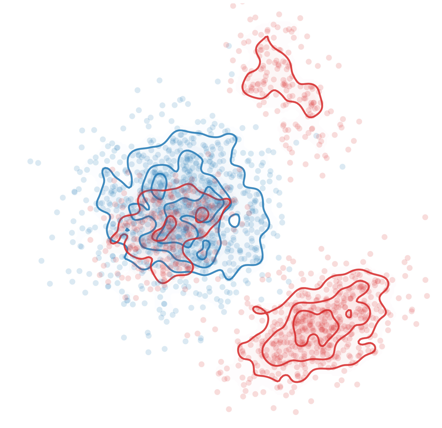
Sample noise x0, data x1, and a shared time pair t < r. Interpolate each endpoint pair at both times to sample pt and pr.
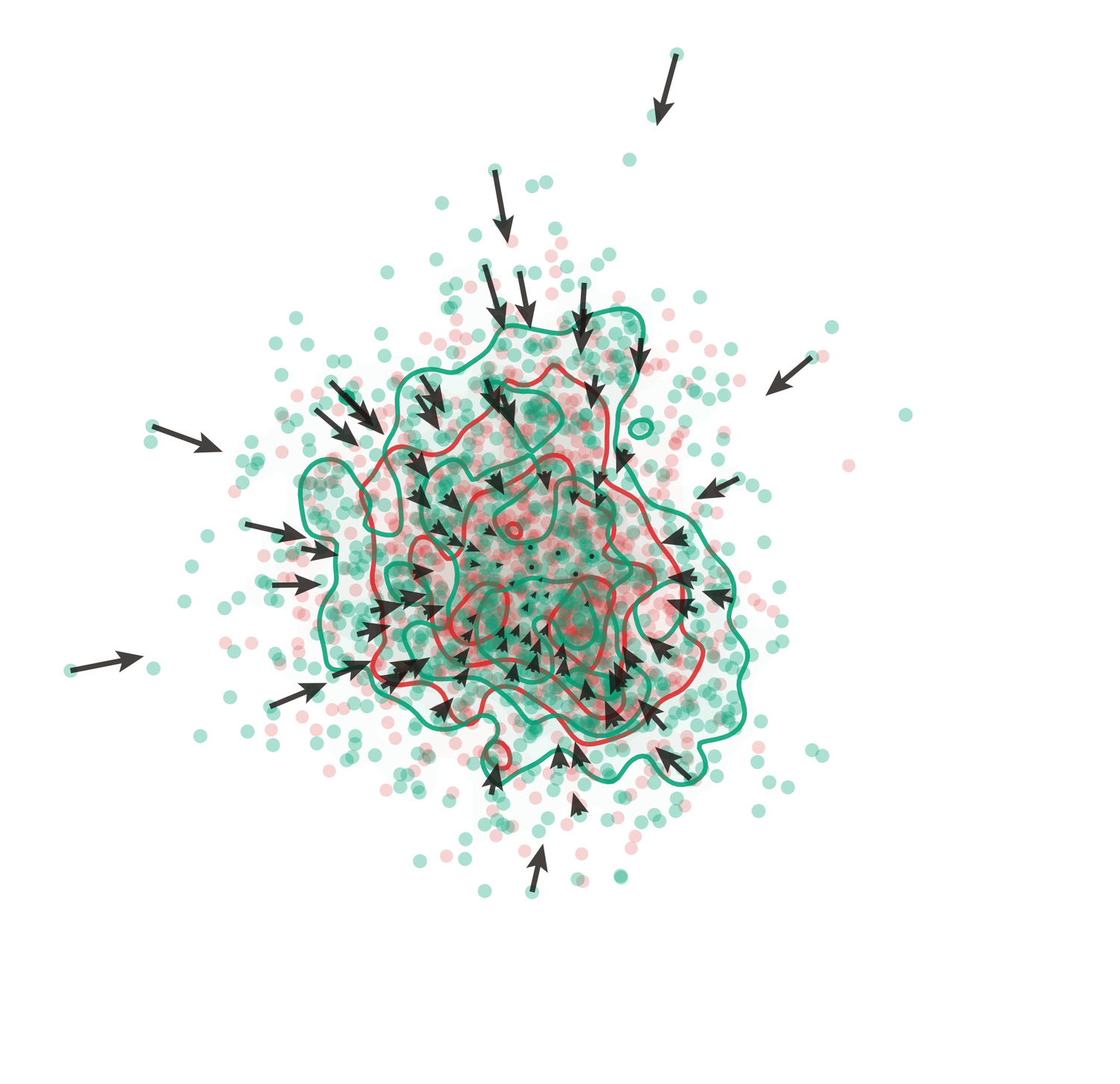
Push samples from pt through the two-time model. Their predicted distribution is qt,r.
Attract predictions toward pr and subtract self-attraction within qt,r. Fit the resulting stop-gradient targets.
xs = (1 − s)x0 + sx1, s ∈ {t, r}
x̂r = xt + (r − t) uθ(xt, t, r)
sg[x̂r + Vq,pᵣ(x̂r)]
DFM learns transport between marginal distributions using a drift objective. Endpoint pairs construct the path samples; the loss matches their distributions within each time-pair group.
Each time pair defines its own marginal transport problem. Compute drift within that group, using the grouped Sinkhorn field in Algorithm 2 of the paper.
At inference
A single interval from 0 to 1 gives direct generation. A finer time grid composes the same learned transport across intermediate states. Each call evaluates the learned mean velocity uθ once.
The constructed marginal path admits explicit Wasserstein bounds. Under the paper’s first-order consistency and regularity assumptions, the learned mean velocity approaches the local Flow Matching velocity as the interval shrinks.
03 / Generation trajectories
A generation trajectory is the sequence of sample states produced during inference. NFE counts model evaluations per sample.
Same method · DFM at 1 NFE and 20 NFE.
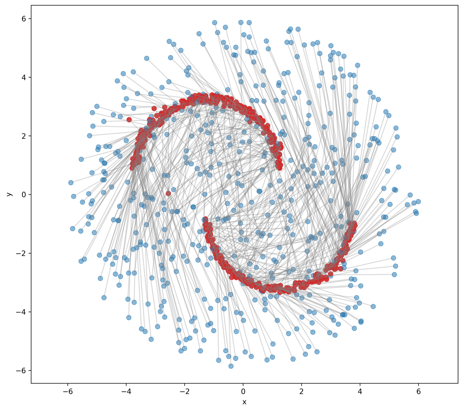
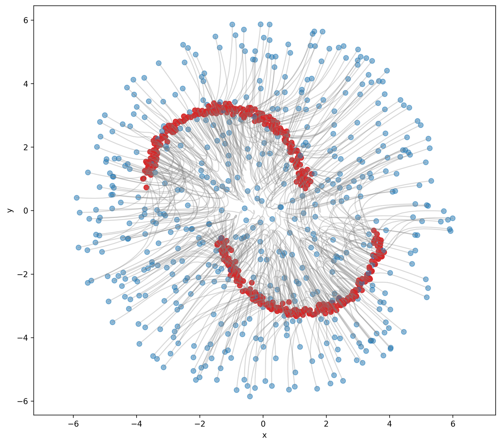
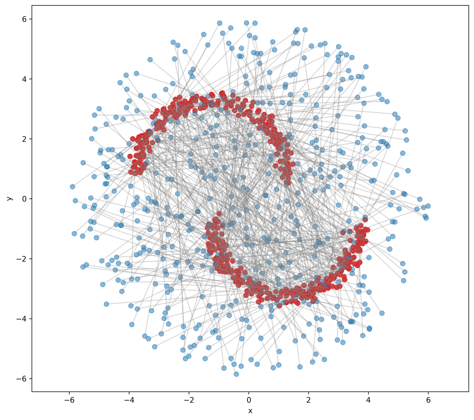
Red endpoints show target samples; lines are reference interpolations.
Blue points show source samples. Red points show generated endpoints in the method panels and target samples in Ground Truth.
04 / Results
The paper evaluates generation quality, distribution coverage, and control success across inference budgets.
116.2 → 80.4 → 75.9
1 → 2 → 5 NFE
Decoded-real reference protocol
1.52 → 1.31
1 → 10 NFE
DFM-L/2 · 463M parameters
0.41 → 0.86
1 → 10 NFE
Average over the last 10 checkpoints
Class-conditional generation on MNIST and FFHQ. EMD is squared Wasserstein-2 distance in latent space. FFHQ FID compares generated and real latents decoded by the same frozen ALAE decoder.
| Method | NFE | MNIST EMD ↓ | MNIST accuracy ↑ | FFHQ EMD ↓ | FFHQ FID ↓ |
|---|---|---|---|---|---|
| Flow Matching | 50 | 37.2 | 100.0% | 198.4 | 77.4 |
| MeanFlow | 1 | 68.6 | 96.7% | 258.7 | 131.2 |
| MeanFlow | 2 | 48.1 | 99.1% | 211.7 | 85.4 |
| MeanFlow | 5 | 37.5 | 100.0% | 204.2 | 82.1 |
| Drift Model | 1 | 37.3 | 100.0% | 225.5 | 116.2 |
| DFM | 1 | 37.3 | 100.0% | 225.5 | 116.2 |
| DFM | 2 | 37.2 | 100.0% | 215.7 | 80.4 |
| DFM | 5 | 37.2 | 100.0% | 196.2 | 75.9 |
More inference steps improve FFHQ latent-space coverage. PCA and UMAP compare the generated and real latent distributions.
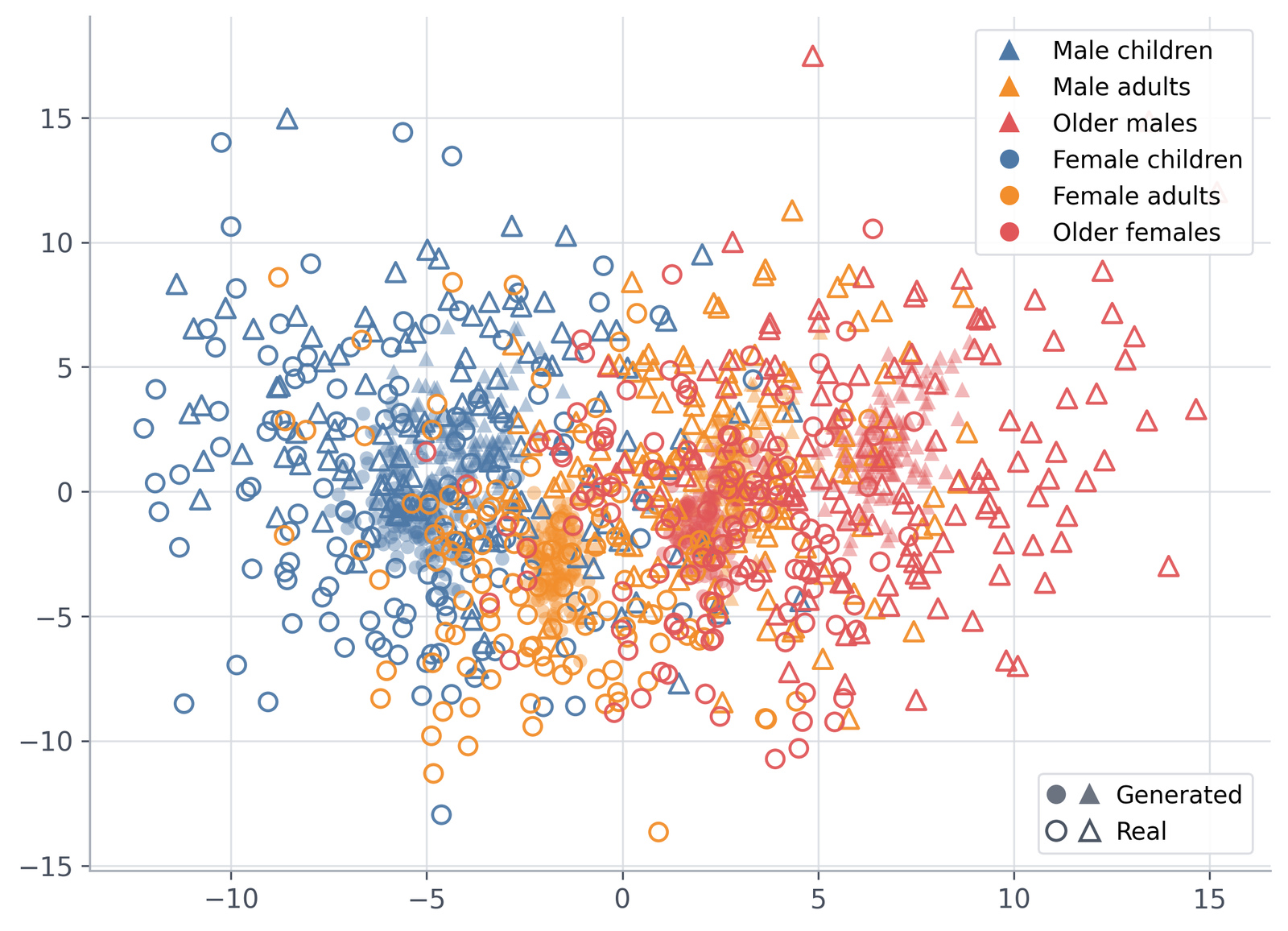
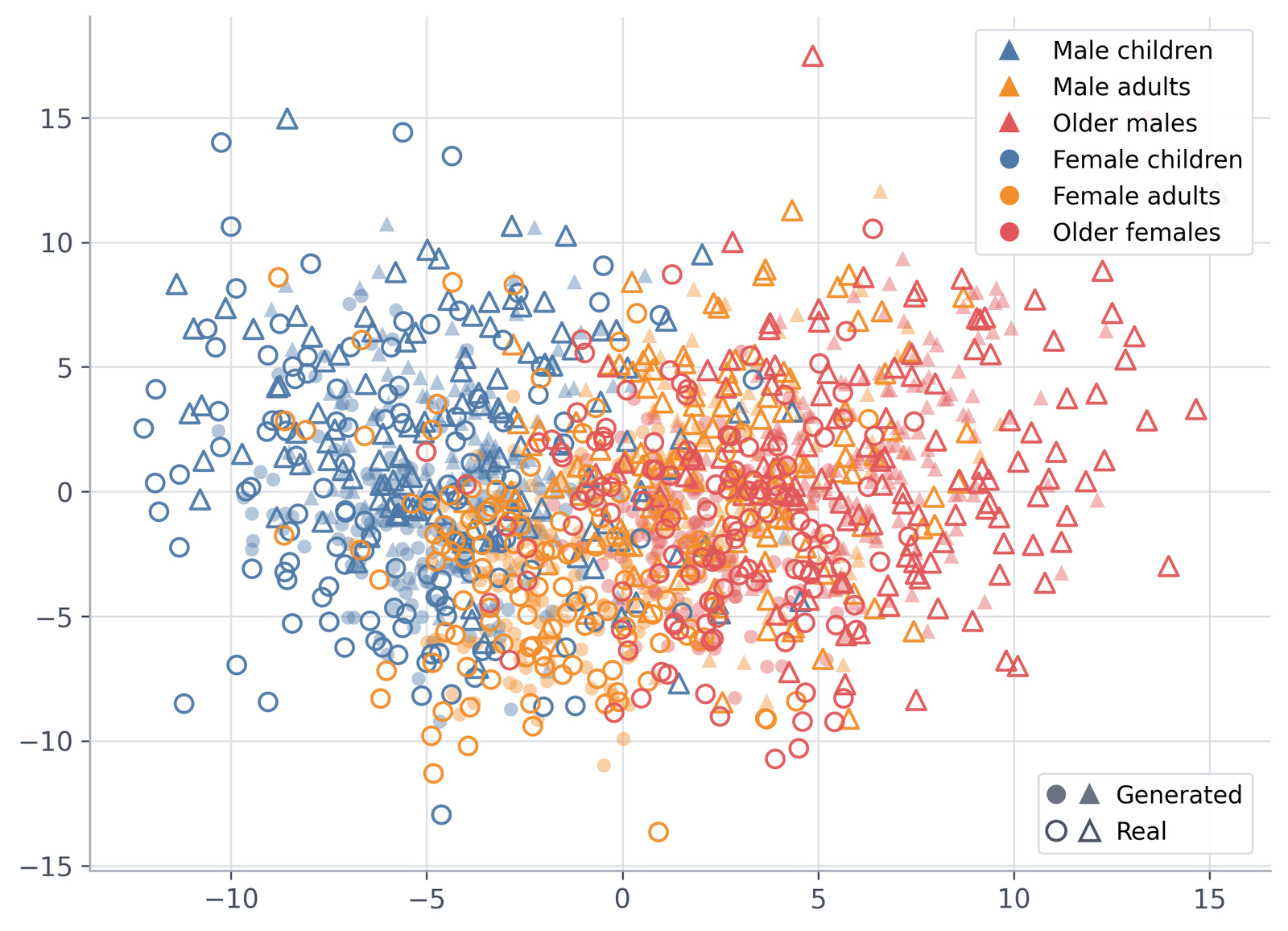
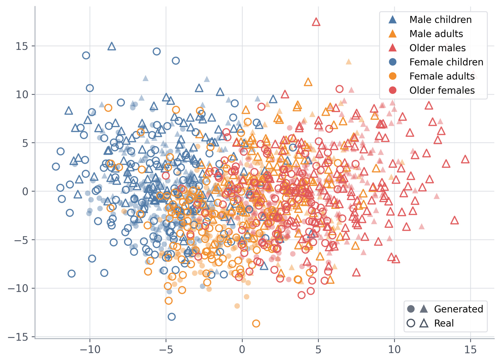
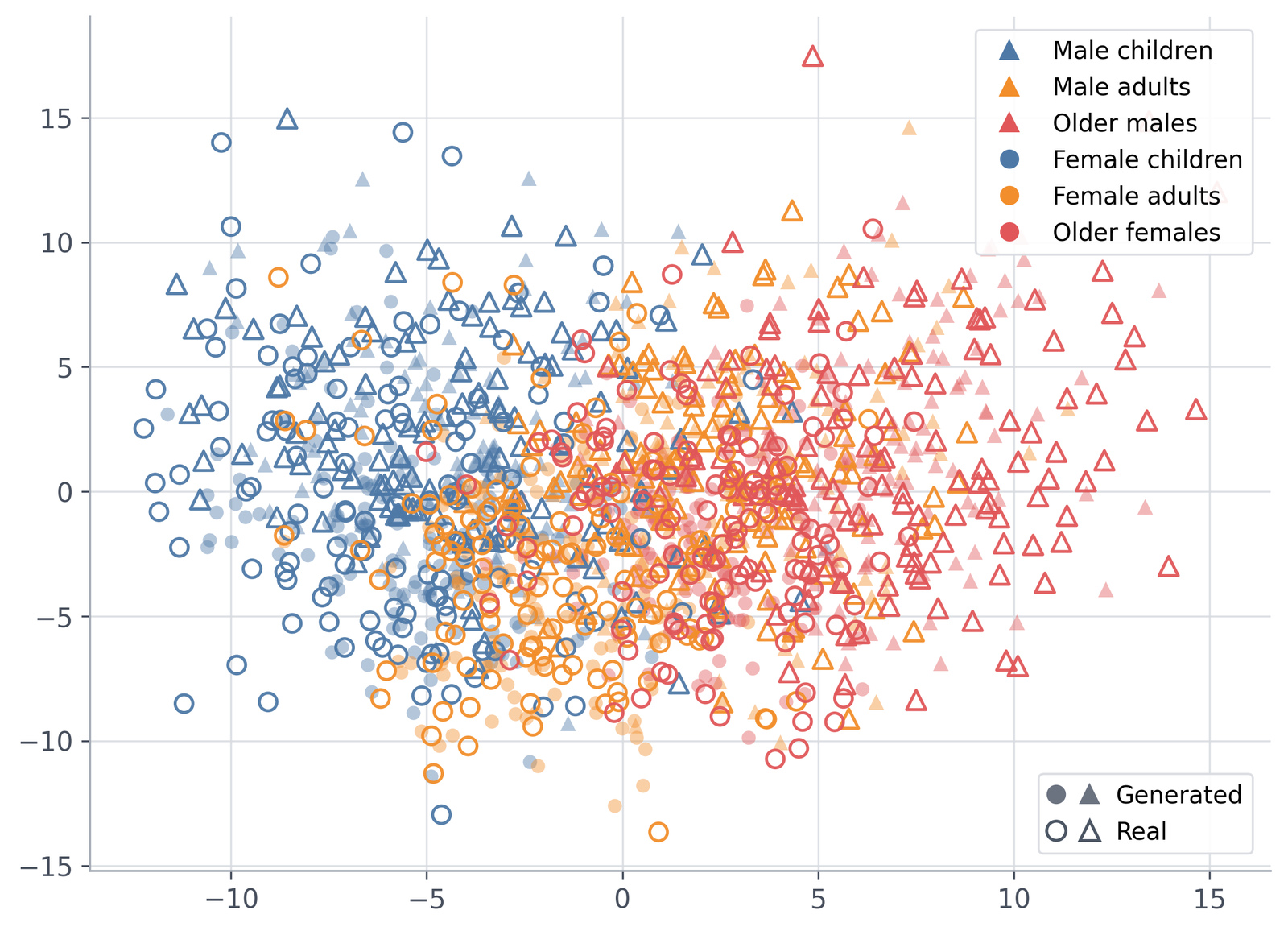
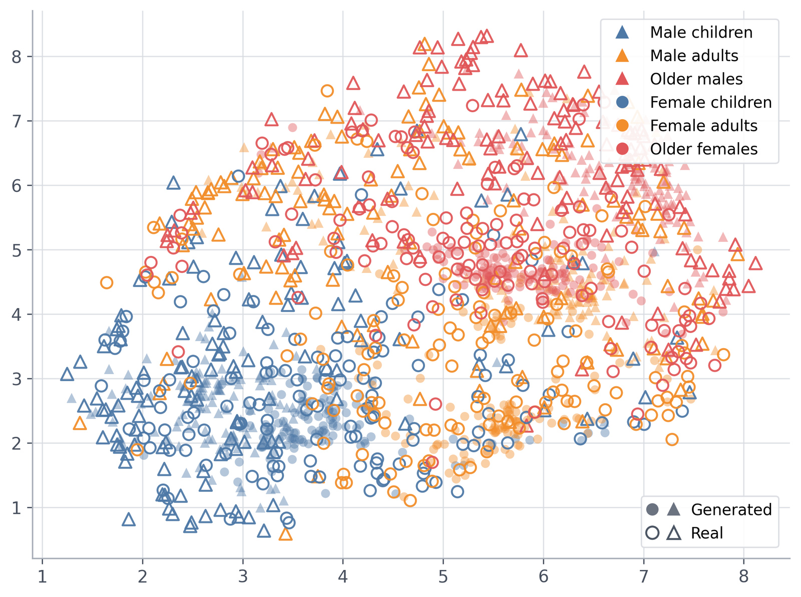
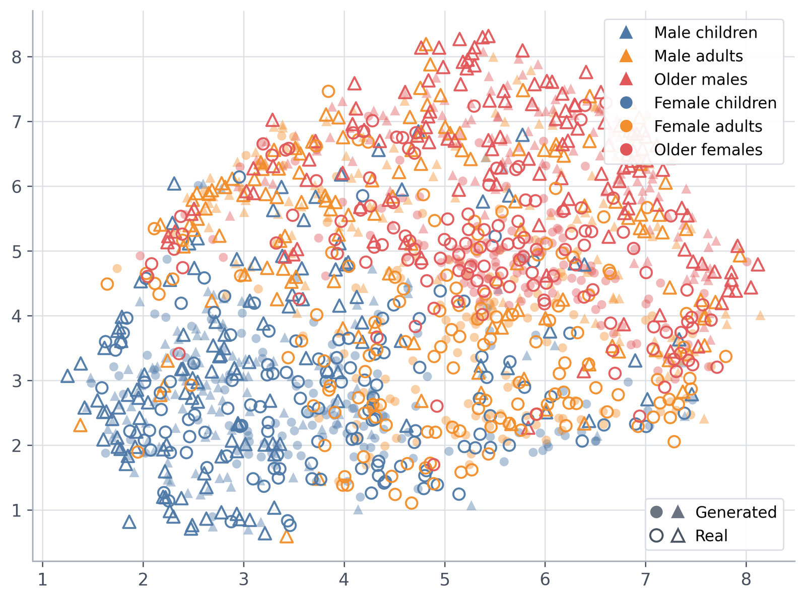
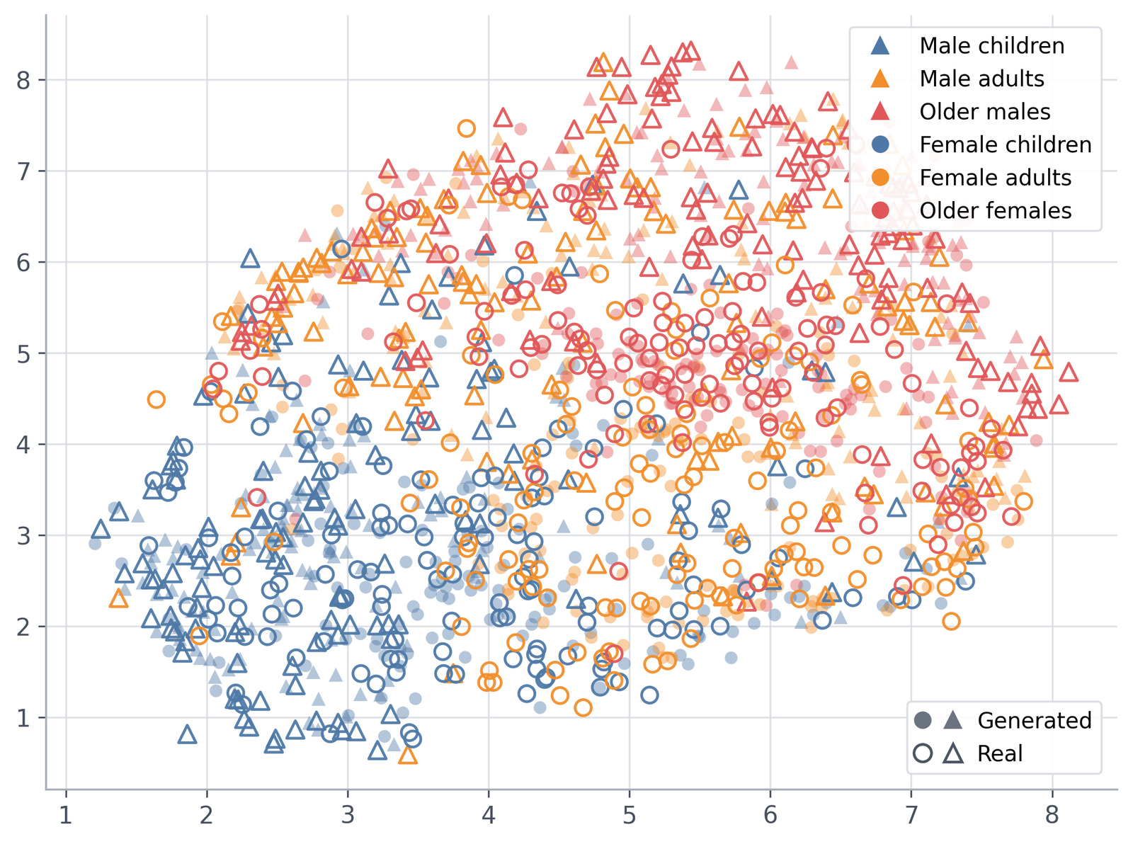
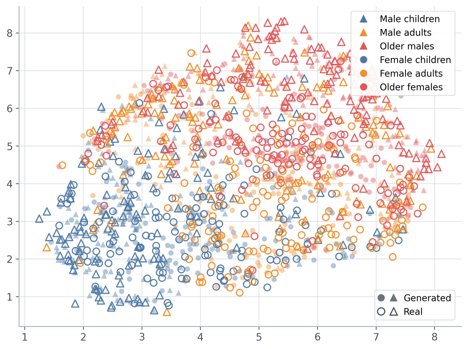
Filled markers show generated latents; outlined markers show real latents. Colors and shapes denote classes.
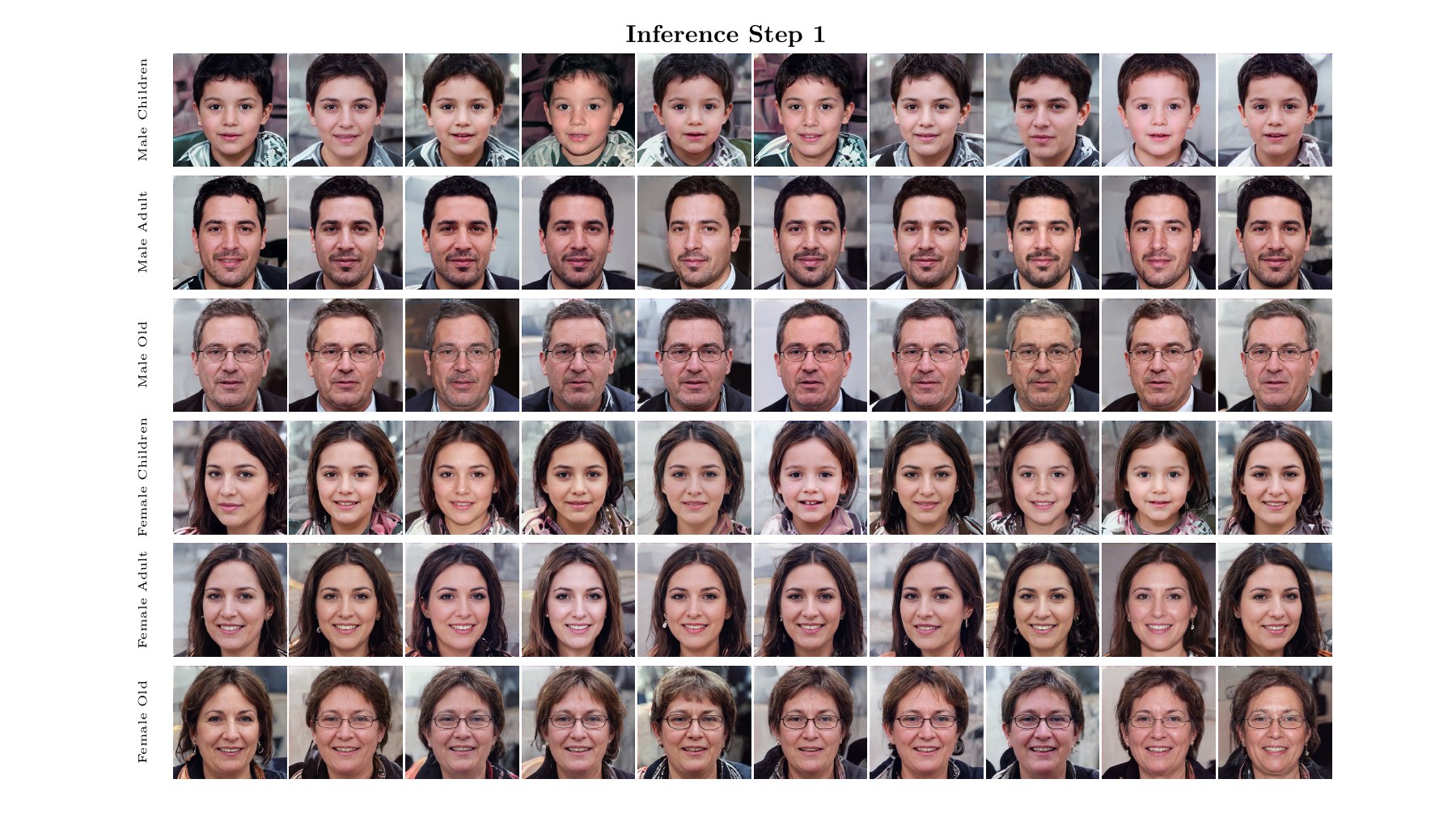
Class-conditional samples from the paper appendix, decoded at 1024 × 1024.
FFHQ · 1 NFE · FID 116.2 · EMD 225.5
The same inference-budget question extends to larger-scale image generation and action generation.
| NFE | FID ↓ | Inception Score ↑ |
|---|---|---|
| 1 | 1.52 | 259.4 |
| 2 | 1.45 | 268.3 |
| 5 | 1.34 | 279.8 |
| 10 | 1.31 | 287.4 |
FID and IS use 50K generated samples in the pretrained VAE latent-space setting.
| NFE | ToolHang · state ↑ | PushT · visual ↑ |
|---|---|---|
| 1 | 0.41 | 0.86 |
| 2 | 0.77 | 0.87 |
| 5 | 0.81 | 0.89 |
| 10 | 0.86 | 0.90 |
Success rates average the last 10 checkpoints.
05 / Code
Prepare MNIST or FFHQ latents, train DFM, sample at a chosen NFE, and evaluate with the documented protocol.
Installation & training →Start with a small CPU example. Train DFM, FM, or MeanFlow, save a model, and record inference trajectories at different budgets.
Run the example →@article{ma2026drift,
title = {Drift Flow Matching},
author = {Ma, Chenrui and Xiao, Xi and Zhao, Lin and Wang, Tianyang
and Fioretto, Ferdinando and Shen, Yanning},
journal = {arXiv preprint arXiv:2605.17244},
year = {2026}
}